1 Introduction

Underwater sound has the potential to affect marine life in different ways depending on its sound level and characteristics. Richardson et al. (1995) defined four zones of sound influence which vary with distance from the source and level. These are:

• The zone of audibility: this is the area within which the animal can detect the sound. Audibility itself does not implicitly mean that the sound will affect the marine life.
• The zone of masking: this is defined as the area within which sound can interfere with the detection of other sounds such as communication or echolocation clicks. This zone is very hard to estimate due to a paucity of data relating to how marine mammals detect sound in relation to masking levels (for example, humans can hear tones well below the numeric value of the overall sound level).
• The zone of responsiveness: this is defined as the area within which the animal responds either behaviourally or physiologically. The zone of responsiveness is usually smaller than the zone of audibility because, as stated previously, audibility does not necessarily evoke a reaction.
• The zone of injury/hearing loss: this is the area where the sound level is high enough to cause tissue damage in the ear. This can be classified as either Temporary Threshold Shift (TTS) or Permanent Threshold Shift (PTS). At even closer ranges, and for very high intensity sound sources (e.g. underwater explosions), physical trauma or even death are possible.

For this study, it is the zones of injury and disturbance (i.e. responsiveness) that are under consideration (there is insufficient scientific evidence to properly evaluate masking). To determine the potential spatial range of injury and disturbance effects from subsea noise, a review has been undertaken of available evidence, including international guidance and scientific literature. The following sections summarise the relevant thresholds for onset of effects and describe the evidence base used to derive them.

This technical note provides details of the proposed noise modelling methodology for piling as part of the Ossian offshore wind farm as follows:

• Proposed injury and disturbance thresholds.
• Pile source level determination.
• Sound propagation modelling methodology.
• Sound exposure calculations.

We anticipate a response to this methodology statement within 28 days of the receipt of this document. Agreement with the approach is to be ideally reached before the modelling commences. Should a response not be received within 28 days, it will be assumed that MD-LOT are in agreement with the method proposed.

The Scoping Opinion has been received and considered in the development of the underwater noise modelling methodology.

2                         Proposed injury and disturbance thresholds

2 Proposed injury and disturbance thresholds

2.1                  Marine mammals

2.1 Marine mammals

Sound propagation models can be constructed to allow the received sound level at different distances from the source to be calculated. To determine the consequence of these received levels on any marine mammals which might experience such sound emissions, it is necessary to relate the levels to known or estimated potential impact thresholds. The auditory injury (PTS/TTS) threshold criteria proposed by Southall et al. (2019) are based on a combination of un-weighted peak pressure levels and marine mammal hearing weighted Sound Exposure Level (SEL). The hearing weighting function is designed to represent the frequency characteristics (bandwidth and sound level) for each group within which acoustic signals can be perceived and therefore assumed to have auditory effects. The proposed PTS and TTS thresholds to be employed for Ossian are summarised in Table 2.1.

Table 2.1:  Summary of PTS and TTS onset acoustic thresholds for impulsive sounds (Southall et al., 2019; Table 6).

Disturbance of marine mammals due to impulsive sound from piling activity will be assessed quantitatively by considering the proportional response of individuals exposed to decreasing sound levels with increasing distance from the sound source. Empirical evidence from piling studies at the Beatrice Offshore Wind Farm (Moray Firth, Scotland) (Graham et al., 2019) and Horns Rev Offshore Wind Farm (Brandt et al., 2011) demonstrated that the probability of occurrence of harbour porpoise Phocaena phocoena (measured as porpoise positive minutes) increased exponentially moving further away from the source. Graham et al. (2019) showed a 100% probability of disturbance at an (un-weighted) SEL of 180  (dB) re 1μPa2s, 50% at 155dB re 1μPa2s and dropping to approximately 0% at an SEL of 120dB re 1μPa2s and the data were subsequently used to develop a dose-response curve.

Similarly, a telemetry study undertaken by Russell et al. (2016) investigating the behaviour of tagged harbour seals Phoca vitulina during pile driving at the Lincs Offshore Wind Farm in the Wash found that there was a proportional response at different received sound levels. Dividing the study area into a 5 km x 5 km grid, the authors modelled SELss levels and matched these to corresponding densities of harbour seals in the same grids during periods of non-piling versus piling to show change in usage. The study found that there was a significant decrease during piling activities at predicted received SEL levels of between 142 and 151 dB re 1 µPa2s.

The approach to be employed for Ossian is therefore to plot un-weighted single pulse SEL contours in 5 dB increments and apply the appropriate dose-response curve to estimate the number of animals that would be disturbed by sound from the piling within each stepped contour. For cetaceans, the dose-response curve will be applied from the Beatrice Offshore Wind Farm data (Graham et al., 2019) whilst for pinnipeds the dose-response curve will be applied using Whyte et al. (2020).

2.2                  Fish, larvae and sea turtles

2.2 Fish, larvae and sea turtles

The injury threshold criteria for fish, larvae and sea turtles used in this underwater sound assessment for impulsive piling are given in Table 2.2. In the table, both peak and SEL criteria are un-weighted. Physiological effects relating to injury criteria are described below (Popper et al., 2014; Popper and Hawkins, 2016):

• Mortality and potential mortal injury: either immediate mortality or tissue and/or physiological damage that is sufficiently severe (e.g. a barotrauma) that death occurs sometime later due to decreased fitness. Mortality has a direct effect upon animal populations, especially if it affects individuals close to maturity.
• Recoverable injury: Tissue and other physical damage or physiological effects, that are recoverable but which may place animals at lower levels of fitness, may render them more open to predation, impaired feeding and growth, or lack of breeding success, until recovery takes place.
• TTS: Short term changes in hearing sensitivity may, or may not, reduce fitness and survival. Impairment of hearing may affect the ability of animals to capture prey and avoid predators, and also cause deterioration in communication between individuals; affecting growth, survival, and reproductive success. After termination of a sound that causes TTS, normal hearing ability returns over a period that is variable, depending on many factors, including the intensity and duration of sound exposure.

Table 2.2:  Criteria for onset of injury to fish and sea turtles due to impulsive piling (Popper et al., 2014).

3                         Pile source level determination

3 Pile source level determination

3.1                  Summary of general concepts

3.1 Summary of general concepts

The sound generated and radiated by a pile as it is driven into the ground is complex, due to the many components which make up the generation and radiation mechanisms. Larger pile sizes can require a higher energy in order to drive them into the seabed, and different seabed and underlying substrate types can require use of different installation techniques including varying the hammer energies and the number of hammer strikes. In addition, the seabed characteristics can affect how sound propagates from the pile through the sub-surface geology, thus fundamentally affecting the acoustic field around the activity. The type of hammer method used (i.e. the force-impulse characteristics) can also affect the sound characteristics.

Underwater sound source level is usually quantified using a dB scale with values generally referenced to 1 μPa pressure amplitude as if measured at a distance of 1 m from a hypothetical, infinitesimally small source (often referred to as the Source Level). This quantity is often referred to as an equivalent monopole source level. In practice, it is not usually possible to measure at 1 m from a large structure, which in reality is more akin to a distributed sound source, but the metric allows comparison and reporting of different source levels on a like-for-like basis. In reality, for a large sound source such as a monopile, this conceptual point at 1 m from the (theoretical, infinitesimally small) acoustic centre does not exist. Furthermore, the energy is distributed across the source and does not all emanate from this imagined acoustic centre point. Therefore, the stated Sound Pressure Level (SPL) at 1 m does not occur at any point in space for these large sources. In the acoustic near field (i.e. close to the source), SPL will be significantly lower than the value predicted by the Source Level.

A useful measure of sound used in underwater acoustics is the SEL. This descriptor is used as a measure of the total sound energy of an event or a number of events (e.g. over the course of a day) and is normalised to one second. This allows the total acoustic energy contained in events lasting a different amount of time to be compared on a like for like basis. The SEL is defined as:

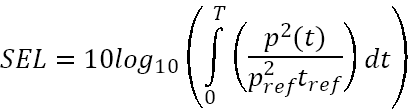
where is the integration time of the sound “event”, is the squared sound pressure at a time and is the reference time-integrated squared sound pressure of 1 µPa2s. For impulsive sounds it has become customary to utilise the T90 time period for calculating and reporting root mean squared (rms) sound pressure levels. This is the interval over which the cumulative energy curve rises from 5% to 95% of the total energy and therefore contains 90% of the sound energy.

3.2                  Proposed pile source modelling methodology

3.2 Proposed pile source modelling methodology

The estimation of source levels for sound propagation modelling of piling is an important aspect of the noise modelling methodology.  Ideally, use can be made of noise data measurement for similar piles, installed using a similar hammer in similar conditions.  However, since noise modelling for proposed wind farms often proposes the use of piles and hammers for which there is no currently available measured data, it is often necessary to utilise an alternative method to estimate the source level inputs to the model. One such method used in some previous noise modelling assessments is the use of energy conversion factors, which involves estimating the proportion of the hammer energy which is transmitted into the water column as sound.  However, the subject of sound generation due to impact piling is an active area of research and the evidence base is constantly being updated by new measurements, research and published papers. It is therefore important to ensure that the methodology used for determining the source levels of piling take into account the most recent research.

It is proposed to utilise scaling of measured data during pile driving for similar operations to Ossian in order to determine source levels. The subject of sound generation due to impact piling is an active area of research and the evidence base is constantly being updated by new measurements, research and published papers.  A recent peer-reviewed paper (von Pein et al., 2022) presents a methodology for the dependencies of the SEL on strike energy, diameter, ram weight, and water depth that can be used for scaling measured or computed SELs from one project to another. The method has been shown to be usable within practical ranges of accuracy, especially if the measurement uncertainties are taken into account. The paper suggests that scaling should be performed over either a small number of very similar piling situations or over a larger data set with according averaging. This is a recently published method for deriving the sound source level which provides a more scientifically robust method compared to using an energy conversion factor (the conversion factor method simply assumes that a percentage of the hammer energy is converted into sound irrespective of parameters such as pile size, water depth and hammer specifications).  Since the von Pein et al. (2022) methodology takes into account several site-specific and pile-specific factors, in addition to hammer energy, and because it is based on a scientifically rigorous and peer reviewed study, it is therefore considered to be a significant improvement on the use of simple conversion factors alone.

Using the equation below (von Pein et al. 2022), a broadband source level value is calculates for the noise emitted during impact pile driving operation in each operation window.

In this equation, E is the hammer energy employed in Joules, d is the pile diameter, mr is the ram mass in kg, h is the water depth in m, is the reflection coefficient and is the propagation angle (approximately 17° for a Mach wave generated by impact piling). The equation allows measured pile noise data from one site (denoted by subscript 0) to be scaled to another site (denoted by subscript 1).

To account for the pile penetration and use of submerged piling rigs, a correction is applied through the piling sequence based on Lippert et al. (2017) by considering the quotient of wetted pile length Lw and water depth hw using the following equation:

This methodology therefore takes into account the following factors:

• Pile diameter
• Pile length.
• Pile penetration.
• Water depth.
• Rated maximum hammer energy of the proposed hammer.
• Hammer energy being used.
• Ram mass for the hammer.
• Acoustical parameters of the soil and water.

The peak SPL can be calculated from SEL values via the empirical fitting between pile driving SEL and peak SPL data, given in Lippert et al. (2015), as:

SPLpk = .

Root mean square (rms) sound pressure levels were calculated assuming a typical T90 pulse duration (i.e. the period that contains 90% of the total cumulative sound energy) of 100 ms. It should be noted that in reality the rms T90 period will increase significantly with distance which means that any ranges based on rms sound pressure levels at ranges of more than a few kilometres are likely to be significant over estimates and should therefore be treated as highly conservative.

The piling scenarios for Ossian have not yet been finalised, but it is envisaged that these will include the following phases:

• Initiation (including slow-start);
• Soft start;
• Ramp up; and
• Full power piling.

Mitigation methods such as use of Acoustic Deterrent Devices (ADDs) and engineering means of reducing sound emissions will be investigated as part of the sound modelling exercise if required.

4                         Sound propagation modelling methodology

4 Sound propagation modelling methodology

There are several methods available for modelling the propagation of sound between a source and receiver ranging from very simple models which simply assume spreading effects according to a 10 log (R) or 20 log (R) relationship (as discussed above, and where R is the range from source) to full acoustic models (e.g. ray tracing, normal mode, parabolic equation, wavenumber integration and energy flux models). In addition, semi-empirical models are available, whose complexity and accuracy are somewhere in between these two extremes.

In choosing the correct propagation model to employ, it is important to ensure that it is fit for purpose and produces results with a suitable degree of accuracy for the application in question, taking into account the context, as detailed in “Monitoring Guidance for Underwater Noise in European Seas Part III”, NPL Guidance, (Dekeling et al., 2014) and in Farcas et al. (2016). Thus, in some situations (e.g. low risk of auditory injury due to underwater sound, where range dependent bathymetry is not an issue, i.e. for non-impulsive sound) a simple (N log R) model might be sufficient, particularly where other uncertainties (such as uncertainties in source level or the impact thresholds) outweigh the uncertainties due to modelling. On the other hand, some situations (e.g. very high source levels, impulsive sound, complex source and propagation path characteristics, highly sensitive receivers, and low uncertainties in assessment criteria) warrant a more complex modelling methodology.

The first step in choosing a propagation model is therefore to examine these various factors, such as:

• Balancing of errors/uncertainties;
• Range dependant bathymetry;
• Frequency dependence; and
• Source characteristics.

For the sound field model, relevant geo-acoustic data, physical parameters and bathymetry will be developed based on a combination of data provided by the Applicant combined with the information gathered from the publicly available literature. These parameters will be fed into an appropriate propagation model routine, in this case the Weston Energy Flux model (for more information see Weston, 1971; 1980a; 1980b), suited to the region and the frequencies of interest. The frequency-dependent loss of acoustic energy with distance (TL) values will then be evaluated along different transects around the chosen source points.

The propagation loss is calculated using one for the four formulae detailed in  Table 4.1, depending on the distance of the receiver location from the source, and related to the frequency and the seafloor conditions such as depth and its composition.

Table 4.1:  Regions of transmission loss derived by Weston (1971).

In Table 4.1, is the depth at the source, is the depth at the receiver, is the minimum depth along the bathymetry profile (between the source and the receiver), is the critical grazing angle (related to the speed of sound in both seawater and the seafloor material), and are the wavelength and wavenumber as usual, and is the seabed reflection loss gradient, empirically derived to be 12.4 dB/rad in Weston (1971).

The spherical spreading region exists in the immediate vicinity of the source, which is followed by a region where the propagation follows a cylindrical spread out until the grazing angle is equal to the critical grazing angle . Above the critical grazing angle in the mode stripping region an additional loss factor is introduced which is due to seafloor reflection loss, where higher modes are attenuated faster due to their larger grazing angles. In the final region, the single-mode region, all modes but the lowest have been fully attenuated.

For estimation of propagation loss of acoustic energy at different distances away from the sound source location (in different directions), the following steps were considered:

• The bathymetry information around this chosen source points will be extracted from the GEBCO database in 72 different transects.
• A geoacoustic model of the different seafloor layers in the survey region will be calculated.
• A calibrated Weston Energy model will be employed to estimate the TL matrices for different frequencies of interest (from 25 Hz to 80 kHz) along the 72 different transects.
• The calculated source level values will be combined with the TL results to achieve a frequency and range dependant RL of acoustic energy around the chosen source position.
• The TTS and PTS potential impact distances for different marine mammal groups will be calculated using relevant metrics and weighting functions (from Southall et al., 2019) and by employing a simplistic animal movement model (directly away from the sound source) where appropriate.
• The Weston model will be calibrated against Parabolic Equation and Normal Mode models.

5                         Sound exposure calculations

5 Sound exposure calculations

As well as calculating the un-weighted instantaneous peak sound pressure levels, it is also necessary to calculate the received acoustic signal in terms of the SEL metric (where necessary and possible) for a marine mammal using the relevant hearing weighting functions. For different operations related sound sources, the numerical SEL value is equal to the SPL rms value integrated over a one second window as the sources are continuous and non-impulsive. These SEL values are employed for the calculation of cSEL (cumulative SEL) metric for different marine mammal groups to assess potential impact ranges. In the case of fish exposure, the exposure calculations are carried out using the unweighted cumulative SEL as per the threshold criteria.

Simplified exposure modelling could assume that the animal is either static and at a fixed distance away from the sound source, or that the animal is swimming at a constant speed in a perpendicular direction away from a sound source. For fixed receiver calculations, it has generally been assumed (in literature) that an animal will stay at a known distance from the sound source for a period of 24 hours. As the animal does not move, the sound will be constant over the integration period of 24 hours (assuming the source does not change its operational characteristics over this time). This, however, would give an unrealistic level of exposure, as the animals are highly unlikely to remain stationary when exposed to loud sound, and are therefore expected to swim away from the source. The approximation used in these calculations, therefore, is that the animals move directly away from the source.

It should be noted that the sound exposure calculations are based on the simplistic assumption that the sound source is active continuously (or intermittently based on source activation timings) over a 24 hour period. The real world situation is more complex. The SEL calculations presented in this study do not take any breaks in activity into account, such as repositioning of the piling vessel, and are therefore likely to be an overestimation.

Furthermore, the sound criteria described in the Southall et al. (2019) guidelines assume that the animal does not recover hearing between periods of activity. It is likely that the intervals between operations could allow some recovery from temporary hearing threshold shifts for animals exposed to the sound (Benda-Beckmann et al. 2022) and, therefore, the assessment of SEL is conservative. 

In order to carry out the moving animal calculation, it has been assumed that an animal will swim away from the sound source at the onset of activities.  For impulsive sounds of piledriving the calculation considers each pulse to be established separately resulting in a series of discrete SEL values of decreasing magnitude (see Figure 5.1).

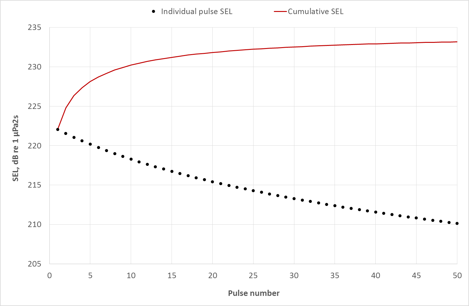
Figure 5.1: A comparison of discrete SEL per pulse, and cumulative SEL values.

As an animal swims away from the sound source, the sound it experiences will become progressively lower (more attenuated); the cumulative SEL is derived by logarithmically adding the SEL to which the mammal is exposed as it travels away from the source. This calculation will be used to estimate the approximate minimum start distance for an animal in order for it not to be exposed to sufficient sound energy to result in the onset of potential auditory injury. It should be noted that the sound exposure calculations are based on the simplistic assumption that the animal will continue to swim away at a fairly constant relative speed. The real-world situation is more complex, and the animal is likely to move in a more complex manner.

The assumed swim speeds for animals likely to be present across the Ossian Marine Mammal Study area are set out in Table 5.1.

Table 5.1: Assessment swim speeds of marine mammals and fish that are likely to occur within the Irish Sea for the purpose of exposure modelling.

To perform the cumulative exposure calculation, the first step is to parameterise the m-weighted sound exposure levels (or unweighted in the case of fish) for single strikes of a given energy via the 95th percentile line of best fit against the calculated received levels from the model. This function is then used to predict the exposure level for each strike in the planned hammer schedule (periods of slow start, ramp up and full power).

6                   Conclusions and next steps

6 Conclusions and next steps

This methodology note has set out the approach that is proposed for modelling subsea noise for Ossian, including:

• Proposed injury and disturbance thresholds, which are based on the latest scientific consensus and peer reviewed papers;
• Pile source level determination methodology, which is based on a peer reviewed method taking into account pile parameters, including pile diameter, pile length, pile penetration depth, water depth, rated maximum hammer energy of the proposed hammer, hammer energy being used, ram mass for the hammer and acoustical parameters of the seabed soil and water.
• Sound propagation modelling methodology, which is based on a peer reviewed method which has been used for modelling of several offshore wind farm developments, including in Scotland, and
• Sound exposure calculation methodology, including the proposed swim speeds, hearing weightings and metrics, all of which are based on the latest scientific evidence.

Proposed next steps in terms of stakeholder engagement on the underwater noise modelling methodology are as follows:

• Stakeholders are requested to review this methodology note and provide any clarification questions or concerns prior to the next meeting.
• RPS and Seiche will then respond to any questions either during the meeting or by issuing a further clarification note.
• Assuming agreement with the approach is reached and any clarifications have been closed out, it is expected that the formal MS-LOT Scoping Opinion will include a relevant statement with regards to the agreed approach.

Agreement with the approach is to be ideally reached before the modelling commences.

7                         References

7 References

Bailey, Helen, Bridget Senior, Dave Simmons, Jan Rusin, Gordon Picken, and Paul M. Thompson. (2010) ‘Assessing Underwater Noise Levels during Pile-Driving at an Offshore Windfarm and Its Potential Effects on Marine Mammals’. Marine Pollution Bulletin 60 (6): 888–97.

Benda-Beckmann, A. M. von, D. R. Ketten, F. P. A. Lam, C. A. F. de Jong, R. A. J. Müller, and R. A. Kastelein. (2022) ‘Evaluation of Kurtosis-Corrected Sound Exposure Level as a Metric for Predicting Onset of Hearing Threshold Shifts in Harbor Porpoises (Phocoena Phocoena)’. The Journal of the Acoustical Society of America 152 (1): 295–301.

Boisseau, Oliver, Tessa McGarry, Simon Stephenson, Ross Compton, Anna-Christina Cucknell, Conor Ryan, Richard McLanaghan, and Anna Moscrop. (2021) ‘Minke Whales Balaenoptera Acutorostrata Avoid a 15 KHz Acoustic Deterrent Device (ADD)’. Marine Ecology Progress Series 667: 191–206.

Brandt, Miriam J., Ansgar Diederichs, Klaus Betke, and Georg Nehls. (2011) ‘Responses of Harbour Porpoises to Pile Driving at the Horns Rev II Offshore Wind Farm in the Danish North Sea’. Marine Ecology Progress Series 421: 205–16.

Dekeling, R. P. A., M. L. Tasker, A. J. Van der Graaf, M. A. Ainslie, M. H. Andersson, M. André, J. F. Borsani, K. Brensing, M. Castellote, and D. Cronin. (2014) ‘Monitoring Guidance for Underwater Noise in European Seas, Part II: Monitoring Guidance Specifications. A Guidance Document within the Common Implementation Strategy for the Marine Strategy Framework Directive by MSFD Technical Subgroup on Underwater Noise.’

Farcas, Adrian, Paul M. Thompson, and Nathan D. Merchant. (2016) ‘Underwater Noise Modelling for Environmental Impact Assessment’. Environmental Impact Assessment Review 57: 114–22.

Graham, Isla M., Nathan D. Merchant, Adrian Farcas, Tim R. Barton, Barbara Cheney, Saliza Bono, and Paul M. Thompson. (2019) ‘Harbour Porpoise Responses to Pile-Driving Diminish over Time’. Royal Society Open Science 6 (6): 190335.

Lippert, Stephan, Marco Huisman, Marcel Ruhnau, Otto von Estorff, and K. van Zandwijk. 2017. “Prognosis of Underwater Pile Driving Noise for Submerged Skirt Piles of Jacket Structures.” In 4th Underwater Acoustics Conference and Exhibition (UACE 2017), Skiathos, Greece.

Lippert, Tristan, Marta Galindo-Romero, Alexander N. Gavrilov, and Otto von Estorff. 2015. “Empirical Estimation of Peak Pressure Level from Sound Exposure Level. Part II: Offshore Impact Pile Driving Noise.” The Journal of the Acoustical Society of America 138 (3): EL287–92.

Otani, Seiji, Yasuhiko Naito, Akiko Kato, and Akito Kawamura. (2000) ‘Diving Behavior And Swimming Speed of a Free-Ranging Harbor Porpoise, Phocoena Phocoena’. Marine Mammal Science 16 (4): 811–14.

Popper, Arthur N., Anthony D. Hawkins, Richard R. Fay, David A. Mann, Soraya Bartol, Thomas J. Carlson, Sheryl Coombs, et al. (2014) ASA S3/SC1.4 TR-2014 Sound Exposure Guidelines for Fishes and Sea Turtles: A Technical Report Prepared by ANSI-Accredited Standards Committee S3/SC1 and Registered with ANSI. Springer.

Popper, A.N. and Hawkins, A.D. (2016). The Effects of Noise on Acquatic Life, II. Springer Science+Business Media. New York, NY.

Richardson, William John, Denis H. Thomson, Charles R. Greene, Jr., and Charles I. Malme. (1995) Marine Mammals and Noise. Academic Press.

Sims, David W., Colin D. Speedie, and Adrian M. Fox. (2000) ‘Movements and Growth of a Female Basking Shark Re-Sighted after a Three Year Period’. Journal of the Marine Biological Association of the United Kingdom 80 (6): 1141–42.

Southall, Brandon L., James J. Finneran, Colleen Reichmuth, Paul E. Nachtigall, Darlene R. Ketten, Ann E. Bowles, William T. Ellison, Douglas P. Nowacek, and Peter L. Tyack. (2019) ‘Marine Mammal Noise Exposure Criteria: Updated Scientific Recommendations for Residual Hearing Effects’. Aquatic Mammals 45 (2): 125–232.

Thompson, D., A. Brownlow, J. Onoufriou, and S. Moss. (2015) ‘Collision Risk and Impact Study: Field Tests of Turbine Blade-Seal Carcass Collisions’. Report to Scottish Government MR 7 (3): 1–16.

von Pein, Jonas, Tristan Lippert, Stephan Lippert, and Otto von Estorff. 2022. “Scaling Laws for Unmitigated Pile Driving: Dependence of Underwater Noise on Strike Energy, Pile Diameter, Ram Weight, and Water Depth.” Applied Acoustics 198: 108986.

Weston, D. E. (1971) ‘Intensity-Range Relations in Oceanographic Acoustics’. Journal of Sound and Vibration 18 (2): 271–87.

Weston, D. E. (1980a) ‘Acoustic Flux Formulas for Range-Dependent Ocean Ducts’. The Journal of the Acoustical Society of America 68 (1): 269–81.

Weston, D. E. (1980b) ‘Acoustic Flux Methods for Oceanic Guided Waves’. The Journal of the Acoustical Society of America 68 (1): 287–96.

Whyte, K., Russell, D., Sparling, C., Binnerts, B. and Hastie, G. (2020). Estimating the effects of pile driving sounds on seals: Pitfalls and possibilities. The Journal of the Acoustical Society of America.