1. Introduction

1. This Benthic Subtidal Ecology Technical Report provides a full benthic subtidal ecology baseline for the Array, using the most contemporary desktop data sources and the results of the 2022 site-specific surveys. This Benthic Subtidal Ecology Technical Report is part of the Array Environmental Impact Assessment (EIA) Report, which has been commissioned for Ossian Offshore Wind Farm Limited (Ossian OWFL).
2. For the purposes of this Array EIA Report, the Array refers collectively to the offshore components of the wind farm (i.e. wind turbines, Offshore Substation Platforms (OSPs), and inter-array and interconnector cables). The Array is situated within the site boundary ( Figure 2.1   Open ▸ ).
3. The site boundary is located in the North Sea, approximately 80 km south-east of Aberdeen, and comprises an approximate area of 859 km2.

2.             Study Area

2. Study Area

4. Two study areas have been defined for the purpose of the benthic subtidal ecology assessment:

• The Array benthic subtidal ecology study area, which is defined as the area encompassed by the site boundary ( Figure 2.1   Open ▸ ). The site-specific benthic subtidal ecology surveys were undertaken within this area, the results of which were used to inform the baseline characterisation and identify benthic receptors which could potentially be impacted by the Array.
• The regional benthic subtidal ecology study area, which is defined as the area encompassing the wider North Sea ( Figure 2.1   Open ▸ ). The boundaries for this regional benthic subtidal ecology study area were adapted from the Sectoral Marine Plan (SMP) Assessment region: East Region. The regional benthic subtidal ecology study area boundary to the south of the site boundary was extended to take account of feedback received during the Scoping Workshop (14 November 2022) requesting that the regional benthic subtidal ecology study area was not large enough to account for both direct and indirect effects. Desktop data sources have been used to characterise the regional benthic subtidal ecology study area, which will, overall, provide wider context to the site-specific data collected within the Array benthic subtidal ecology study area.

Figure 2.1: Benthic Subtidal Ecology Study Areas

3.             Baseline

3. Baseline

3.1.        Methodology

3.1. Methodology

5. A desktop review and the results of site-specific surveys have been used to inform the baseline for benthic subtidal ecology in the Array EIA Report. These desktop data sources include academic literature, reports from other developments within the regional benthic subtidal ecology study area (e.g. Berwick Bank Offshore Wind Farm, Seagreen Offshore Wind Farm, etc.) and governmental reports. Two site-specific surveys were undertaken for the Array in 2022: a geophysical survey and an environmental survey ( Table 3.5   Open ▸ ). Detailed methodologies are provided in sections 3.2.1 and 3.2.2.

3.2.        Desktop Study

3.2. Desktop Study

6. A detailed desktop review of existing studies and datasets was undertaken to gather information on benthic subtidal ecology within the regional benthic subtidal ecology study area. Table 3.1   Open ▸ .summarises the studies and datasets used.
7. Whilst there is an abundance of data sources highlighted in Table 3.1   Open ▸ , many of them target areas further inshore or other offshore wind farms, with less site-specific information on the Array benthic subtidal ecology study area available. However, the site-specific geophysical and environmental surveys are sufficient to characterise the Array benthic subtidal ecology study area in the absence of extensive desktop data sources.

Table 3.1: Summary of Key Desktop Reports

3.2.1.    Regional Benthic Subtidal Ecology Study Area

3.2.1. Regional Benthic Subtidal Ecology Study Area

                        Subtidal sediments

8. The EUSeaMap broadscale substrate data indicates that the regional benthic subtidal ecology study area is dominated by deep circalittoral sand (A5.27; biotope classification: SS.SSa.OSa) and is interspersed with deep circalittoral coarse sediment (A5.15; SS.SCS.OCS) (EMODnet, 2019) ( Figure 3.1   Open ▸ ). Deep circalittoral mud (A5.37; SS.SMu.OMu) and circalittoral mixed sediments (A5.44; SS.SMx.CMx) are mainly present along the coast and within the Firth of Forth. These four sediment classifications are identified as low energy habitats and are considered characteristic of the North Sea (EMODnet, 2019).
9. There are a range of designated sites within the regional benthic subtidal ecology study area which also provide valuable baseline information (refer to section 3.2). For example, the Firth of Forth Banks Complex Marine Protected Area (MPA) displays a mosaic of different sands and gravels, which are influenced by strong currents. Despite these sand and gravel sediments being common in the northern North Sea, the dynamic currents within this MPA influence their distribution to create a unique range of habitats (JNCC, 2014; JNCC, 2021). Video and still photography surveys within the MPA identified three broad habitat types: soft sediments with ripples, mixed sediment, and coarse sediments with some rocky outcrops (Axelsson et al., 2014). The Wee Bankie moraine formation within the Firth of Forth Banks Complex MPA comprises prominent (20 m high) submarine glacial ridges with poorly sorted sediments, such as boulders, gravels, clays and sands (JNCC, 2021).
10. Similarly, site-specific surveys conducted for other offshore wind farm projects within the regional benthic subtidal ecology study area also provide information to support the baseline. An overview of the subtidal sediments identified in these surveys is illustrated in Figure 3.1   Open ▸ . It should be noted that since conducting their site-specific surveys in 2011, the Seagreen Alpha and Seagreen Bravo projects were combined to form Seagreen 1 and Seagreen 1A. The boundary of the whole Seagreen area was changed in the process, so Table 3.2   Open ▸ refers to the superseded Seagreen Alpha and Seagreen Bravo areas to more accurately portray the spatial variation in the data that were collected at the time.

Figure 3.1: Subtidal Sediments within the Regional Benthic Subtidal Ecology Study Area (Source: EMODnet, 2019)

Table 3.2: Overview of Benthic Subtidal Sediments from Other Offshore Wind Farm Projects within the Regional Benthic Subtidal Ecology Study Area

Subtidal benthic communities

11. The results of eight Ministry of Agriculture, Fisheries and Food (now DEFRA, Department for Environment, Food and Rural Affairs) surveys conducted between 1980 and 1985, and the 1986 North Sea Benthos Survey were analysed by Heip and Craeymeersch (1995). The benthic macrofaunal species with the highest frequencies of occurrence in the North Sea are the bristleworm Spiophanes bombyx, polychaetes Pholoe sp., spotted chevron worm Goniada maculata, brittlestar Amphiura filiformis, and catworm Nephtys hombergii (Heip and Craeymeersch, 1995). The diversity of molluscs and crustaceans in the North Sea was highest at a latitude of 56º North (thus within the regional benthic subtidal ecology study area and in line with the Array benthic subtidal ecology study area) (Heip and Craeymeersch, 1995). Conversely, the diversity of annelids and echinoderms in the North Sea was highest from 57º to 60º North, and thus partly overlapping with the regional benthic subtidal ecology study area.
12. More recently, as part of the Regional Seabed Monitoring Programme (RSMP), Cooper and Barry (2017) describe results of the baseline assessment of the UK’s macrobenthic infauna. Although the study was focussed on the aggregates industry, a “big data” approach was taken which collated data from across UK waters, including within the regional benthic subtidal ecology study area. This data was collated from various industries, including offshore wind farms, oil and gas, nuclear and port and harbour sectors. Cooper and Barry (2017) categorised benthic macrofaunal communities into broad groups, based on similarities in their community composition.
13. No RSMP infaunal samples have been taken within the Array boundary itself, however there were some approximately 30 km to the west of it (Cefas 2023; Cooper and Barry 2017). The sample from the dataset were characterised by deep circalittoral sands and deep circalittoral coarse sediment and associated benthic infaunal communities of polychaetes (D2b, D2c and D2d faunal groups: Spionidae, Nephtydae, Lumbrineridae, Oweniidae, Cirratulidae, Capitellidae, Ampharetidae, Opheliidae and Magelonidae), bivalve molluscs (D2b and D2d faunal groups: Semelidae and Tellinidae) and nemerteans (D2b faunal group). Elsewhere in the regional benthic subtidal ecology study area, the Cooper and Barry (2017) dataset presents a mixture of deep circalittoral sands with deep circalittoral coarse sediment and associated benthic infaunal communities of polychaetes (C1a and C1b faunal groups: Spionidae, Glyceridae, Terebellidae, Capitellidae and Phyllodocidae) and nemerteans (D2a faunal group). Within the Firth of Forth, deep circalittoral mud is present, which is associated with infaunal Nephtyidae communities (faunal group D2c: Nephtyidae, Spionidae and Ophelidae).
14. These findings are in line with those of Sotheran and Crawford-Avis (2014) who identified Marine Nature Conservation Review (MNCR) habitats from samples within the regional benthic subtidal ecology study area. S. bombyx aggregations in offshore sands (SS.SSa.OSa.[Sbom]) were identified in deep circalittoral sand. S. bombyx aggregations in offshore coarse sands (SS.SCS.OCS.[Sbom]) and polychaete-rich Galathea communities with encrusting bryozoans and other epifauna on offshore coarse sediments (SS.SCS.OCS.[PoGintBy]) were identified in deep circalittoral coarse sediments.
15. Similarly, Pearce et al. (2014) identified Ross worm Sabellaria spinulosa on stable circalittoral mixed sediment (SS.SBR.PoR.SspiMx), polychaete-rich Galathea communities with encrusting bryozoans and other epifauna on offshore circalittoral mixed sediment (SS.SMx.OMx.[PoGintBy]), and both SS.SSa.OSa.[Sbom] and SS.SCS.OCS.[Sbom], within the regional benthic subtidal ecology study area, albeit further inshore. In a more recent study, Pearce and Kimber (2020) idenitifed the presence of Ross worm off the coasts of Peterhead and Fraserburgh (Aberdeenshire), which are approximately 100 km north of the Array. However, given that the majority of the data presented in Pearce and Kimber (2020) are out with the regional benthic subtidal ecology study area, this study has not been used further to characterise the Array.
16. As stated in paragraph 9, there are a range of designated sites within the regional benthic subtidal ecology study area which provide information about the benthic environment. A 2011 survey within the Firth of Forth Banks Complex MPA described 12 biotopes with a circalittoral muddy sand (SS.SSa.CMuSa) biotope complex being the most commonly recorded (Axelsson et al., 2014). The SS.SSa.CMuSa biotope complex was comprised of two biotopes, one dominated by the bivalves Abra alba and Nucula nitidosa, and the other by brittlestar Acronida brachiata and sea star Astropecten irregularis (Axelsson et al., 2014). Mixed sediment habitats (consisting of gravel, sand, mud and some shell material) were typically dominated by brittlestars Ophiothrix fragilis and Ophiocomina nigra, bryozoan Flustra foliacea, or the horse mussel Modiolus. The soft coral, dead man’s fingers Alcyonium digitatum, and ascidians were typically present in coarser sediments (a mixture of gravel, pebbles and cobble overlying finer sediments) (Axelsson et al., 2014).
17. Furthermore, site-specific surveys conducted for other offshore wind farm projects within the regional benthic subtidal ecology study area also provide information to support the baseline. An overview of the subtidal benthic communities recorded in these surveys is presented in Table 3.3   Open ▸ . As per paragraph 10, the superseded names for Seagreen 1 and Seagreen 1A (Seagreen Alpha and Seagreen Bravo) are referred to, in order to more accurately portray the spatial distribution of the data that were collected at the time.

Table 3.3: Overview of Benthic Subtidal Communities from Other Offshore Wind Farm Projects within the Regional Benthic Subtidal Ecology Study Area

3.2.2.    Array Benthic Subtidal Ecology Study Area

3.2.2. Array Benthic Subtidal Ecology Study Area

                        Subtidal sediments

18. The EUSeaMap broadscale substrate data indicate that the sediments within the Array benthic subtidal ecology study area are almost entirely represented by deep circalittoral sand (A5.27; SS.SSa.OSa). There is one small area comprised of deep circalittoral coarse sediment (A5.15; SS.SCS.OCS) located within the north-west of the area ( Figure 3.2   Open ▸ ).

Figure 3.2: Broadscale Subtidal Sediments within the Array Benthic Subtidal Ecology Study Area (Source: EMODnet, 2019)

                        Subtidal benthic communities

19. The NBN Atlas collates species records and presents them spatially on an interactive map for users to explore. Using the NBN Atlas (2021) to explore the Array benthic subtidal ecology study area, the following species were recorded:

• ocean quahog Arctica islandica;
• gastropod Colus gracilis;
• red whelk Neptunea antiqua;
• prickly cockle Acanthocardia echinata;
• dark necklace shell Euspira fusca; and
• horse mussel.

20. These six molluscs were all recorded during dredging surveys conducted by the Conchological Society of Great Britain and Ireland. These surveys have been conducted since 1876, with these particular recordings within the Array benthic subtidal ecology study area dating from 1980 to 2016 (Conchological Society of Great Britain and Ireland, 2023).
21. Otherwise, there are currently few data sources characterising the subtidal benthic communities within the Array subtidal ecology study area itself, with the majority of sources focussed on elsewhere in the regional benthic subtidal ecology study area (as presented in section 2). Therefore, the subtidal benthic communities within the Array subtidal ecology study area will largely be informed by the results of the site-specific environmental survey (refer to section 2).

3.2.3.    Designated Sites

3.2.3. Designated Sites

22. While the Array benthic subtidal ecology study area does not overlap with any protected sites that have been designated for benthic subtidal features, numerous sites occur within the regional benthic subtidal ecology study area. These include an MPA and three Special Areas of Conservation (SACs). Sites of Special Scientific Interest (SSSIs) have not been listed here due to their distance from the Array benthic subtidal ecology study area and their intertidal features which would not be impacted by the Array. For example, the closest SSSIs with benthic ecological designations are the Tayport Tentsmuir Coast SSSI (124.03 km), Berwickshire Coast Intertidal SSSI (126 km), and the Firth of Forth SSSI (126.99 km), which are designated for mudflats, saline lagoons and rocky shores.
23. Using publicly available data supplied by the JNCC, EMODnet, and the Marine Scotland NMPi maps, there are no known Annex I sandbanks, mudflats, reefs, shallow inlets or bays, submerged or partially submerged sea caves, estuaries, or Oslo and Paris Convention (OSPAR) listed threatened and declining habitats overlapping with the Array benthic subtidal ecology study area. As indicated in Figure 3.3   Open ▸ , the closest designated site with benthic subtidal ecology features is the Firth of Forth Banks Complex MPA, which is located at least 25 km from the Array benthic subtidal ecology study area at its closest point. All other designated sites are much further away (i.e. >100 km) and are therefore unlikely to be affected by the Array ( Table 3.4   Open ▸ ).

Table 3.4: Summary of Designated Sites with Relevant Benthic Qualifying Features

Figure 3.3: Designated Sites in Proximity to the Array Benthic Subtidal Ecology Study Area

3.3.        Site-Specific Surveys

3.3. Site-Specific Surveys

24. Table 3.5   Open ▸ provides a summary of the site-specific surveys undertaken to inform the baseline characterisation for benthic subtidal ecology.

Table 3.5: Summary of Surveys Undertaken to Inform the Baseline Characterisation for Benthic Subtidal Ecology

3.3.1.    Methodology

3.3.1. Methodology

25. The following paragraphs describe the methodology for the site-specific environmental survey conducted in 2022. Detailed methodology for the geophysical survey is detailed in the physical processes EIA chapter of the Array EIA Report (volume 2, chapter 7), and are only briefly summarised here:

• Bathymetric data was collected using Multibeam Echosounder (MBES) in order to determine topography and gradients.
• High resolution Side Scan Sonar (SSS) data was collected to determine seabed features, such as high level sediment composition (based upon seabed texture) and the presence of boulders and debris.
• High resolution Sub-Bottom Profiler (SBP) data was collected to determine the subsurface stratigraphy and high level composition, such as the presence of boulders and shallow geological features or hazards, that may influence foundation design.
• Multichannel Two-Dimensional (2D) Ultra High Resolution Seismic (UHRS) data was collected to determine the deeper sub-surface soil conditions that may influence foundation depth.
• Dual magnetometer data across the site to support Unexploded Ordnance (UXO) interpretation and to identify any additional potential hazards or ferrous contacts.

                        Sample collection

26. The site-specific geophysical and environmental surveys were undertaken by Ocean Infinity, using the Motor Vessel (M/V) Northern Maria between March and July 2022. The sampling sites for the environmental survey were informed by preliminary interpretation of the data collected during the geophysical survey, in order to collect samples that provide a representational analysis of the Array benthic subtidal ecology study area.
27. The environmental survey was conducted to ground-truth the geophysical survey data and to identify potential ecological constraints for the Array. The environmental survey consisted of the following, which are discussed in further detail in the subheadings below:

• Drop Down Video (DDV);
• macrofaunal and physico-chemical grab sampling (including sampling for Particle Size Analysis (PSA)); and
• epibenthic beam trawls.

28. The environmental sampling scope involved a multidimensional approach, which included visual inspection (e.g. photographs or video) prior to any grab sampling. Photographs and videos were taken at locations characterised by hard substrates and/or sensitive habitats, whereas grab sampling took place in more homogenous areas alongside visual inspection. A summary of the environmental survey specifications is presented in Table 3.6   Open ▸ and the sampling locations are presented in Table 3.4   Open ▸ .

                        DDV

29. To ensure adequate data coverage of infaunal and epifaunal communities, a total of 80 sampling locations were selected for grab sampling and DDV ( Table 3.4   Open ▸ ). The DDV imagery was collected using a SeaSpyder High Definition (HD) camera system. Prior to conducting the grab sampling, the DDV camera system was deployed at each sampling site and a minimum of five photographs were taken, alongside continuous video footage. Photographs were taken at the centre of each proposed grab sampling site, as well as approximately 10 m north, east, south and west of this centre location. The photographs and video footage collected provided further information on the habitats and the extent of any features identified.
30. The photographs were reviewed by the onsite benthic ecologist in order to confirm the presence or absence of any potentially sensitive habitats and/or features of conservation interest (such as Annex I reefs) prior to conducting any grab samples.

                        Grab sampling

31. The 80 macrofaunal and PSA grab samples were collected using a mini Hamon grab (0.1 m2), and the ten grab samples for contaminants were collected using a Day grab (0.1 m2). According to guidelines by Davies et al. (2001) and Worsfold and Hall (2010), a minimum sediment volume of 7 l is required for macrofaunal analysis and 2.7 l for PSA. Therefore, the minimum grab sample volume required was 7 l; if the sample volume was below 7 l but exceeded 3 l then it was considered acceptable for PSA.
32. The grab samplers were inspected between attempts to ensure that there were no defects which would prevent valid sample collection and to ensure that they were free from residual sediment from previous deployments. Each sampling site was attempted up to three times; if the first attempt was not acceptable (i.e. too low a sample volume, malfunction of the grab sampler, etc.) then up to two re-attempts were made. After three failed attempts, the survey moved on to the next sampling site. Samples that were not acceptable were not included in any analyses, but were used as guidance when assigning habitat types, when applicable.
33. At each sampling site, 1 l of sediment was taken from the sample bucket for PSA in a laboratory. A sub-sample was taken from these PSA samples for Total Organic Carbon (TOC) and Total Organic Matter (TOM) analyses. The remaining sample material was then decanted and sieved using a 5 mm sieve over a 1 mm sieve. A preliminary description and documentation of characteristic fauna was recorded before the samples were preserved in ethanol and stored for further sorting and identification in a laboratory.
34. Grab samples for sediment contamination analysis were collected at ten of the 80 sampling sites (S002, S009, S010, S021, S027, S031, S040, S051, S054 and S068) ( Table 3.4   Open ▸ ). As stated in paragraph 31, these were collected with a Day grab; this is to obtain an undisturbed surface sample which is not possible when using a mini Hamon grab. The grab sampler was cleaned between samples and sample locations. Sediments were collected using a plastic spoon for metals and a metal spoon for organics, hydrocarbons, organotins, and polychlorinated biphenyls (PCBs) to minimise contamination risk. Similarly, samples for metal analysis were stored in a one litre plastic container, and those for organics, hydrocarbons, organotins and PCBs were stored in a 250 ml tin container. The containers were labelled with a unique identification number and frozen according to the laboratory’s recommendations.

                        Epibenthic beam trawls

35. A 2 m beam trawl was used to conduct ten 200 m long trawls for approximately five minutes each. The locations of each trawl are presented in Table 3.4   Open ▸ . The beam trawl had a 22 mm nylon mesh body and a 5 mm mesh (knot to knot) liner in the cod-end, which allowed sampling of small size classes of fish and epifauna. For protection, the belly of the trawl was covered with a chafer net. For optimal fishing efficiency, the trawl was fitted with a 6 mm chain footrope with rubber discs and a single tickler chain. The survey vessel maintained an approximate speed of 1.5 kt to 2 kt for the duration of the trawl.
36. The catch of each trawl was transferred to a container and the net was checked for any remaining organisms. Large debris was removed, and the total catch was photographed before sorting on board the vessel. Fish species were separated from epifaunal invertebrates, and both were divided into species groups, identified to species level and counted. All sample specimens were documented on board, and larger fauna were weighed and measured. All sample specimens were then preserved until they could be delivered to the laboratory; large fauna were frozen and smaller fauna were preserved in ethanol.

Table 3.6: Environmental Survey Specifications

Figure 3.4: Grab and Beam Trawl Sampling Sites

                        Data limitations

37. Macrofaunal samples from grab sampling sites S007, S008, S018, S023, S025, S029, S038, S042, S049, S052 and S070 comprised insufficient sample volume, due to the presence of cobbles, and were excluded from macrofaunal statistical analyses. Similarly, grab sampling site S044 was also excluded from analysis as it was aborted due to camera issues. Sample number S008 had a rock caught in the jaw of the grab, resulting in sample washout on the first and third attempts made, whilst the second attempt contained too low of a volume. Sample number S025 also contained low volume, despite three attempts, likely due to cobbles just below the sediment surface. S008 and S025 were therefore excluded from both the macrofaunal and sediment statistical analyses.

                        Sample analysis

                        Macrofaunal analysis

38. The macrofaunal analyses were conducted by APEM Limited and in accordance with the North East Atlantic Marine Biological Analytical Quality Control (NMBAQC) guidance (Worsfold and Hall, 2010). In the laboratory, the macrofauna were sorted from sediment residue and identified to the lowest taxonomic level possible. Infaunal and non-colonial epifauna were combined and analysed together. Colonial epifauna were recorded as present/absent and analysed separately. If the species was unknown but separate from any other specimens within the same genus, it was assigned a ‘Type’ denomination (e.g. Type A or Type B). Juveniles were marked with the ‘juvenile’ denomination and were excluded from statistical analyses.
39. The epibenthic fauna from the beam trawls were also identified to the lowest taxonomic level possible, with Cnidaria and Nemertea combined into the group ‘Others’ for the phyletic composition analysis. Colonial epifauna from the beam trawls was recorded as present/absent and analysed separately.
40. Biomass analysis was conducted on the grab sample macrofauna, using the blotted wet-weight method, to the nearest 0.0001 g. Biomass for smaller specimens from the beam trawls was also measured using the blotted wet-weight method to the nearest 0.0001 g, where applicable. Larger specimens were weighed to the nearest gram.

                        PSA

41. The PSA was conducted by Kenneth Pye Associates Limited (KPAL). Up to 1 l of sediment from each sampling site was analysed, using a combination of sieving and sedimentation methods. The PSA samples were analysed in accordance with NMBAQC guidelines (Mason, 2022).
42. Samples were wet separated at 2 mm, with the fraction >2 mm analysed using British Standard nested sieves at ‘half’ phi intervals. The <2 mm fraction (0.04 µm to 2 mm) was analysed using laser diffraction. These data for the two fractions were mathematically merged and calculation of particle size summary parameters were calculated using GRADISTAT software (Blott and Pye, 2001). The particle size summary parameters included percentages of mud, sand, and gravel, silt to clay ratio, and sand to mud ratio.
43. The particle sizes were grouped into five large textural groups:

• boulders/cobbles;
• gravel;
• sand;
• silt; and
• clay.

                        Sediment contamination

44. The contaminant analyses were conducted by SOCOTEC. The sediment samples were analysed for the following contaminants: metals, organics (TOM and TOC), hydrocarbons (Total Hydrocarbons (THC) and Polycyclic Aromatic Hydrocarbons (PAHs)), organotins (Dibutyltin (DBT) and Tributyltin (TBT)), and PCBs. The metals analysed were: aluminium (Al), arsenic (As), barium (Ba), cadmium (Cd), chromium (Cr), copper (Cu), iron (Fe), lead (Pb), mercury (Hg), nickel (Ni), vanadium (V) and zinc (Zn).

                        Data analysis

                        DDV

45. The photographs and video stills were analysed to identify species, densities, and seabed substrate, while the video footage was used to aid the assessment of features and habitats. As per Gubbay (2007) and Irving (2009), particular attention was paid to habitats that were elevated above ambient sea level as well as their spatial extent, percentage of biogenic cover, and degree of patchiness, as these are key criteria for evaluating reef structures and areas of conservation importance.
46. The photographs were analysed in terms of individuals per square metre and percentage cover of colonial species. AutoCAD Map Three-Dimensional (3D) was used to count epibenthic fauna and log the scientific name, position, date, time and image ID.

                        PSA

47. The data collected by the methodology described in paragraphs 41 and 42 were used to calculate sediment particle size distribution statistics for each sample. These results were analysed in the Plymouth Routines in Multivariate Ecological Research (PRIMER) v7.0 statistical package (Clarke and Gorley, 2015) and normalised before being included in any statistical analyses. The main sediment fractions and percentages were analysed in a cluster analysis, using the Euclidian distance, and were plotted to examine changes in sediment composition across the Array benthic subtidal ecology study area. A Principal Component Analysis (PCA) was also undertaken on this sediment data to identify spatial patterns and relationships. These data were also used to inform the habitat assessment.

                        Sediment chemistry analysis

48. As there are currently limited UK-specific environmental quality standards for metals and hydrocarbons in sediments, the following assessment criteria and guidelines were used:

• assessment criteria from the Canadian Council of Ministers of the Environment (CCME): the Interim Sediment Quality Guidelines (ISQG) and Probable Effect Level (CCME, 1995; 2001);
• Cefas action levels for disposal of dredged material (Marine Management Organisation (MMO), 2015);
• the OSPAR environmental assessment criteria for metal and PAH concentrations (OSPAR, 2012);
• condition classes established by the Norwegian Environmental Agency (NEA) for contamination in coastal sediments (NEA, 2016, revised 2020); and
• Dutch Rijksinstituut voor Volksgezondheid en Milieu (RIVM) intervention levels for THC concentrations in aquatic sediments (Hin et al., 2010).

49. Threshold values and/or standards are presented within the results in section 3.3.2 for sediment contaminants (refer to Table 3.9   Open ▸ ).

                        Macrofaunal analysis

                        Univariate analysis

50. The PRIMER v7.0 statistical package was used to undertake univariate analysis. The analyses were based on the macrofaunal data from the taxonomic analyses of one replicate from each grab sampling site. This analysis included abundance, number of taxa, Margalef’s index of richness, Pielou’s index of evenness, the Shannon-Wiener diversity index, and the Simpson’s index of dominance. Abundance was expressed as the number of individuals per 0.1 m2 in each grab sample, and the number of taxa was the total number of taxa present in each grab sample.

                        Multivariate analysis

51. As above for the univariate analyses, multivariate analyses were also undertaken using the PRIMER v7.0 statistical package (Clarke and Gorley, 2015), and based on macrofaunal data derived from taxonomical analyses of one replicate from each grab sample site. Abundance was also expressed as the number of individuals per 0.1 m2. The faunal composition was linked to physical variables, such as sediment composition and depth.
52. Macrofaunal specimens were separated into non-colonial and sessile colonial fauna. All colonial fauna was treated separately in the analyses and considered as epifauna. Juvenile specimens, incomplete specimens (e.g. fragments), and protists (such as Ciliophora and Foraminifera) were not included in the analyses. A clustering analyses using the Bray-Curtis similarity coefficient was used to compare faunal composition between sampling sites.
53. In conjunction with the cluster analysis, Non-Metric Multi-Dimensional Scaling (NMDS) was also undertaken. Plotting the NMDS data allows visualisation of relative similarity between sampling sites (i.e. the closer they are, the more similar the species composition between the samples is).
54. Further, a Similarity Proofing Algorithm (SIMPROF) was run in conjunction with the cluster analysis, which was used to identify significantly different naturally occurring groups among grab samples. The SIMPROF test is based on the abundance of taxa in each sample. A Similarity Percentage (SIMPER) analysis was performed on non-transformed data, in order to obtain dissimilarities between groups and to identify the most important percentage contribution seen in the Bray-Curtis similarities.

                        Habitat classification

55. Habitat classification was based on a combination of biotype descriptions from the grab samples (e.g. species abundance, diversity, depth and seabed features), videos and photographs from each sampling site. Habitats were then classified to the lowest hierarchic level possible, using the European Nature Information System (EUNIS) classification (European Environment Agency, 2022).

                        Protected habitat and species assessments (including Annex I reef assessment)

56. As stated in paragraph 30, video footage was obtained at each sampling site to determine whether any sensitive habitats or habitats of special conservation interest were present, to prevent grab sampling of sensitive features. Annex I reefs (code: 1170) were among these habitats. However, the characterisation of what is considered a ‘reef’ is not precise, particularly in relation to colonies of S. spinulosa (a tube-building polychaete) and stony reefs. For example, if S. spinulosa or horse mussel is observed in an area, it is not automatically an Annex I biogenic reef (1170).
57. Thus, a scoring system based on a series of physical, biological and spatial characteristic reef features was established to assess the presence and degree of Annex I reefs (hereafter referred to as the degree of ‘reefiness’). Threshold ranges for this assessment are based on Gubbay (2007), which was further modified by Collins (2010)), and in Irving (2009) ( Table 3.7   Open ▸ and Table 3.8   Open ▸ ).
58. In addition to the Annex I reef assessment, the Scottish Biodiversity List (SBL) (NatureScot, 2020) and the list of Scottish Priority Marine Features (PMFs) (Tyler-Walters, 2016) were consulted to identify species and habitats that have high priority for conservation.

Table 3.7: S. spinulosa Reef Structure Matrix (Step 1) and Reef Structure Matrix vs. Area (Step 2) used to Determine Final ‘Reefiness’ (Source: Collins, 2010, Modified from Gubbay, 2007)

Table 3.8: Guidelines Used to Categorise the Resemblance of Stony Reefs (Source: Irving, 2009)

3.3.2.    Results

3.3.2. Results

                        Geophysical survey

59. As per paragraph 25, seafloor interpretation was based on the SSS and MBES data and aided the characterisation of the seabed sediments within the Array benthic subtidal ecology study area through DDV and grab sampling. The water depth ranged between 63.82 m and 88.66 m, with generally increasing depth from the north-west to the south-east of the Array benthic subtidal ecology study area ( Figure 3.5   Open ▸ ). The bathymetry of the Array benthic subtidal ecology study area consists of gentle slopes which generally deepen towards the east, with larger sediment features running in a north/south direction and small sediment features running in a more east/west direction ( Figure 3.5   Open ▸ and Figure 3.6   Open ▸ ). The seafloor gradient was very gentle, with occasional higher slope angles and very steep slopes observed on wrecks.
60. Consistent with the results of EUSeaMap data, the subtidal sediments observed during the site-specific geophysical survey of the Array benthic subtidal ecology study area are dominated by sand (EMODnet, 2019). However, there were larger and more numerous patches of gravel and occasional diamicton (poorly sorted mixed sediments), including boulder fields, observed, mainly in the west ( Figure 3.7   Open ▸ ). The results of the geophysical survey therefore indicate a slightly less homogenous sediment composition than the broadscale EUSeaMap data ( Figure 3.2   Open ▸ ), which is typically expected when drawing comparisons between broadscale interpolated data and detailed site-specific information. The widespread presence of megaripples and sand waves indicated some sediment mobility, while occasional furrows, mainly in the west of the Array benthic subtidal ecology study area, were indicative of erosion ( Figure 3.6   Open ▸ ).

                        Seabed sediments and sediment composition

                        Particle size distribution

61. The subtidal benthic sediments recorded during the environmental survey were classified into sediment types according to the Folk (1954) classification. The PSA results demonstrated that the sediment composition across the Array benthic subtidal ecology study area had limited variation, mainly comprising of sand with a few sites revealing higher gravel content. The dominating sediment fraction was sand, with a mean content of 86.4% (Standard Deviation (SD) = ±9.8). The mud content was low overall, with a mean content of 9.1% (SD = ±3.6), comprising 8% silt (SD = ±3.3), and 1.2% clay (SD = ±0.4). Gravel content was low, yet variable, with a mean content of 4.5% (SD = ±10.2). Mud typically increased towards the south-eastern end of the Array benthic subtidal ecology study area, with areas of coarser sediments (gravel and gravelly sand) mainly present in the north-west. The sediment fractions for each of the grab sampling sites is presented in full in volume 3, appendix 8.1, annex A.

Figure 3.5: Bathymetry within the Array Benthic Subtidal Ecology Study Area

Figure 3.6: Surficial Geology and Seabed Features within the Array Benthic Subtidal Ecology Study Area

Figure 3.7: Sediment Features and Boulder Fields within the Array Benthic Subtidal Ecology Study Area

                        Multivariate sediment analysis

62. As stated in paragraph 37, grab samples S008 and S025 were excluded from statistical analyses due to insufficient sample volumes. Thus, 78 samples were included in the SIMPROF analysis, which generated 26 distinct groups ( Figure 3.8   Open ▸ ). Principle Component 1 (PC1) (explaining 65.1% of the variation) separated the sampling sites based on the sand to gravel ratio. Principle Component 2 (PC2) (explaining 36.7% of the variation) separated the sampling sites based on the mud content ( Figure 3.9   Open ▸ ).
63. SIMPROF groups b, d and t comprise mixed sediment composition, corresponding to the Folk class Gravelly Muddy Sand. Groups c, e, f, g, h, i, j, k, l, m and n comprise sand with a noticeable mud content, corresponding to the Folk classes Muddy Sand, and Slightly Gravelly Muddy Sand. Groups o, p, q, r, s, u, v, w, x, y and z comprise sand with low gravel and mud content, corresponding to the Folk classes Gravelly Sand, Slightly Gravelly Sand, and Sand. Group a comprises coarse material, corresponding to Folk classes Sandy Gravel.

Figure 3.8: Dendrogram Based on Euclidian Distance for the Sediment Composition for the 78 Suitable Samples, Showing SIMPROF Groups with a 5% Significance Level

Figure 3.9: PCA Plot of Sediment Composition for the 78 Suitable Samples, Showing Sediment Groups Based on the Folk Classification

                        Organic content

64. Organic content can provide an indication of the influence of organic enrichment of the seabed sediment and the activity of primary producers (e.g. phytoplankton). TOM and TOC refer to the amount of organic matter preserved within the sediment.
65. TOM and TOC levels varied across the Array benthic subtidal ecology study area and were both generally higher in the southern and eastern areas. There was an average TOM content of 0.8% (SD=0.3) and average TOC content of 0.2% (SD=0.1) (full details are provided in volume 3, appendix 8.1, annex A).

                        Sediment contamination

                        Metals

66. Concentrations of metals varied little across the Array benthic subtidal ecology study area and were low overall. As presented in Figure 3.9   Open ▸ , threshold values were only exceeded at one sampling site (S002). At this sampling site, an As level of 16.70 µg/g was recorded. This exceeded the NEA 2 Good threshold (15 µg/g) and the CCME ISQG threshold (7.24 µg/g) but is below the Cefas AL1 threshold of 20 µg/g, as illustrated by the highlighted cells in Figure 3.9   Open ▸ .

Table 3.9: Summary of Metal Concentrations (µg/g Dry Weight) in Sediment, Together with Threshold Values. Highlighted Cells Indicate Where Threshold Values Have Been Exceeded

*Not included in statistical analyses of mean, SD, minimum, maximum, and median.

                        Organotins (DBT and TBT)

67. Ten grab samples were tested for organotins. Organotins are endocrine disruptors and are considered one of the most toxic chemicals in the marine environment (Roark, 2020). Levels of both DBT and TBT were below the limit of detection (<1 µg/kg) at all ten sampling sites.

                        Hydrocarbons (THC and PAHs)

68. THC concentrations varied across the Array benthic subtidal ecology study area and were generally higher in the southern and eastern areas, with a peak of 13,700 µg/kg. They did not exceed any of the Dutch RIVM intervention levels at any of the sampling sites ( Table 3.10   Open ▸ ). To provide context, a study by Harries et al., (2001) which examined levels of THC between 1975 and 1995 from oil and gas surveys found that levels of THC located over 5 km from platforms (considered background levels) across the North Sea were 25,500 µg/kg (95th percentile; i.e. greater than 95% of all survey values included).
69. PAH concentrations were low overall, but variable across the Array benthic subtidal ecology study area, with concentrations higher in the southern and eastern areas to a maximum of 81.20 µg/kg at S051 based on the full suite of two to six ring PAHs. This is within the range typically expected in offshore marine sediments in the North Sea which broadly extends from approximately 28 µg/kg to 200 µg/kg (OSPAR, 2000). There were no threshold values exceeded for individual PAHs but the sum of the Environmental Protection Agency (EPA) 16 group exceeded the lower threshold value for NEA 2 Good at S051 ( Figure 3.10   Open ▸ ). Full details are provided in volume 3, appendix 8.1, annex A.

Figure 3.10: Levels of EPA 16 PAH Congeners Summarised Against the Threshold Values for NEA 2 Good (30 µg/kg Dry Weight)

Table 3.10: Summary of Alkane Concentrations (µg/kg Dry Weight) Across the Grab Sampling Sites

                        PCBs

70. PCBs are toxic compounds which are persistent in the environment and are known to bioaccumulate (Kodavanti and Loganathan, 2014). Levels of all 25 PCB congeners tested were below the limit of detection (<0.08 µg/kg) at all ten sampling sites.

                        Macrofaunal grab sample analysis

                        Non-colonial fauna

71. The phyletic composition of the non-colonial fauna identified from the grab sampling is presented in Table 3.11   Open ▸ . Annelida had the highest abundance and diversity, followed by Arthropoda and Mollusca, with these three phyla contributing to 88% of the recorded taxa and 89% of the individuals. The ten most abundant non-colonial fauna identified are presented in Table 3.12   Open ▸ . The most abundant and frequently occurring species were the sand mason worm Lanice conchilega, the bristleworm S. bombyx, and the elongated furrow shell Abra prismatica.
72. Biomass of the non-colonial fauna was grouped into Echinodermata, Mollusca, Annelida, Arthropoda, Nemertea, Sipuncula and ‘O. The group ‘Other’ included Phoronida, Cnidaria, Hemichordata, Platyhelminthes, Chaetognatha and Nematoda. The non-colonial fauna species biomass was expressed as blotted wet weight (g per 0.1 m2) and is illustrated in Figure 3.11   Open ▸ and Figure 3.12   Open ▸ , and provided in full in volume 3, appendix 8.1, annex A.
73. The biomass was dominated by Echinodermata, with 65% of the total biomass, although just one individual of the burrowing sea urchin Spatangus purpureus constituted 19% of the total Echinoderm weight. The second largest group was Mollusca (28%), followed by Annelida (6%) and Nemertea (1%) and ‘Other’ (<1%).
74. Non-colonial fauna biomass varied between 0.13 g/0.1 m2 in sample S064 and 61.94 g/0.1 m2 in sample S061. The mean biomass across all sites was 7.01 g/0.1 m2 (SD = ±13.95) (see volume 3, appendix 8.1, annex A for further information).
75. One specimen of the ocean quahog was found at the location S013 with shell dimensions of 7 cm x 6 cm x 4 cm. As this species is listed as a PMF in Scottish waters, this identified specimen was returned to sea and not incorporated in the total biomass composition.

Table 3.11: Phyletic Composition of Non-Colonial Fauna from the Grab Samples

Table 3.12: Ten Most Abundant and Frequently Occurring Taxa Identified from the Grab Samples

Figure 3.11: Total Biomass (Blotted Wet Weight in g/0.1 m2) Composition of Major Non-Colonial Fauna

Figure 3.12: Total Biomass (Blotted Wet Weight in g/0.1 m2) of ‘Other’ Non-Colonial Fauna

                        Sessile colonial fauna

76. A total of four major sessile colonial phyla and 26 different taxa were identified from the macrofaunal grab samples. Cnidaria was the dominant phylum, contributing to 54% of the total taxa. Bryozoa followed, accounting for 31%, followed by Entoprocta (11%) and Porifera (4%) ( Table 3.13   Open ▸ ; Figure 3.13   Open ▸ ). Bryozoa were the most abundant, followed by Cnidaria and Entoprocta, and only one colony of Porifera was identified ( Table 3.13   Open ▸ ; Figure 3.14   Open ▸ ).

Table 3.13: Phyletic Composition of Sessile Colonial Fauna from Macrofaunal Grab Samples

Figure 3.13: Diversity of Sessile Colonial Fauna Identified from Macrofaunal Grab Samples

Figure 3.14: Abundance of Sessile Colonial Fauna Identified from Macrofaunal Grab Samples

                        Univariate statistical analyses

77. Univariate analyses were performed to assess the richness, diversity, evenness and dominance of the non-colonial fauna. The results of the univariate analysis for each grab sampling site are provided in full in volume 3, appendix 8.1, annex A.
78. Overall, the mean number of taxa per site was 23 (SD = ± 5.35) and varied from 14 (at S004) to 34 (at S055). The mean number of individuals per site (expressed per 0.1 m2) was 69 (SD = ±23.84) and varied between 28 individuals (at S063) to 143 individuals (at S010).
79. The species richness measured with Margalef’s diversity index varied between 3.38 and 8.14, with grab sample S074 having the highest richness. Pielou’s evenness index ranged from 0.69 to 0.95, the Shannon-Wiener index varied from 1.99 to 3.19 and the Simpson’s index of dominance ranged from 0.76 to 0.95; site S077 revealed the highest value for all three parameters.

                        Multivariate statistical analyses

80. A square root transformation was applied to the non-colonial macrofaunal dataset before calculating the Bray-Curtis similarity matrix. This transformation was applied to prevent abundant species from influencing the similarity index measures excessively and to take rarer species into account (Clarke and Gorley, 2015). The SIMPROF analysis of the square rooted non-colonial macrofaunal dataset produced five statistically distinct groups, with the majority of sampling sites in group e, as illustrated in Figure 3.15   Open ▸ .
81. Sample similarity across all sampling sites was further assessed using the NMDS plot presented in Figure 3.16   Open ▸ . This plot reflects the dendrogram in Figure 3.15   Open ▸ and displays the similarity between sampling sites at 30%, to highlight species compositions. The similarity explored in the NMDS plot presented a relatively high stress value of 0.27 suggesting a relatively poor representation of the data. These results were indicative of homogeneity between sampling sites.

Figure 3.15: SIMPROF Dendrogram Based on Square Root Transformed Non-Colonial Faunal Composition from Macrofaunal Grab Sampling Sites

Figure 3.16: NMDS Plot Based on Square Root Transformed Non-Colonial Faunal Composition from Macrofaunal Grab Sampling Sites

82. A SIMPER test was conducted using the results of the Bray-Curtis similarities test (paragraph 80), and is presented in Figure 3.14   Open ▸ . Average abundance refers to square root transformed data and is expressed per 0.1 m2 within the multivariate groups.

Table 3.14: Summary of Characteristics of Non-Colonial Faunal Groups Derived from the SIMPER Test Performed on the Square Rooted Dataset

83. The relationship between PSA and non-colonial macrofaunal communities was assessed by applying the Biota-Environment Matching and Stepwise Test (BEST) analysis within PRIMER. This BEST analysis identifies which of the sediment variables best explain the macrofaunal distribution observed. The results indicated that two variables, gravel and mud, constituted the best-explained pattern of spatial distribution for non-colonial fauna and were statistically significant variables (rho = 0.29, p = 0.01).
84. Bray-Curtis similarity measures in the SIMPER and SIMPROF analyses were also applied to the untransformed non-colonial macrofaunal dataset, as the largest abundances were typically <20 individuals per sampling site ( Figure 3.17   Open ▸ ). There were two statistically distinct groups produced in the SIMPROF analysis and the NMDS plot presented a stress value of 0.21 ( Figure 3.17   Open ▸ and Figure 3.18   Open ▸ ). Like the square root transformed dataset, these results were also indicative of homogeneity between sampling sites, although the stress value indicates a moderate representation of the data within the plot. A SIMPER test was also conducted on the untransformed dataset with species abundance for each SIMPROF group and is presented in volume 3, appendix 8.1, annex A.
85. It should be noted that slight differences were observed between the Ocean Infinity and RPS SIMPER and SIMPROF analyses on the untransformed data. Ocean Infinity reported three statistically distinct groups, opposed to the two identified by RPS, despite using an identical raw data spreadsheet. The discrepancy only involved sampling site S063, which was reported as the third statistically distinct group by Ocean Infinity. As site S063 had the lowest number of individuals in the dataset, and all stations revealed generally low numbers of individuals overall, this discrepancy is likely due to minor test parameter differences between the two analyses. However, as there were no discrepancies between the analyses on the square root transformed dataset, this discrepancy observed in the untransformed analyses is considered of negligible importance.

Figure 3.17: SIMPROF Dendrogram Based on Untransformed Non-Colonial Faunal Composition from Macrofaunal Grab Sampling Sites

Figure 3.18: NMDS Plot Based on Untransformed Non-Colonial Faunal Composition from Macrofaunal Grab Sampling Sites

                        Epibenthic fauna from DDV and still photography

86. Analysis of the DDV and photography showed that the habitats were generally dominated by sand and muddy sand with occasional shell debris, cobbles and pebbles. Generally, the faunal presence in the imagery was sparse, and mainly comprised of L. conchilega, Paguridae, the bryozoan F. foliacea, Tubularia sp., and scattered colonies of Epizoanthus sp. Cnidarians and annelids were conspicuous, mostly associated with areas of sandy substrate. There were three sites with no fauna recorded (S012, S026, and S064), and consisted of sand or muddy sand with occasional shell debris present. The average number of species per site was four, and the highest number of taxa (n=17) was recorded at S066 ( Table 3.15   Open ▸ ). The ten sites with the highest number of taxa recorded are presented in .

Table 3.15: Top Ten DDV and Photography Sampling Sites with the Greatest Diversity of Taxa

Figure 3.19: Photograph from Sampling Site S066, showing Circalittoral Fine Sand with Caridae, Paguridae, Gastropoda, Urticina sp., Idotea sp. and Scalpellum sp.

                        Non-colonial epifauna from seabed photographs

87. The most abundant phylum in the photographs was Annelida, which represented 39% of all individuals recorded, with the majority of recordings represented by L. conchilega (38%) and the remaining 1% comprised of Aphrodita aculeata, Spirobranchus triqueter, Serpulidae and Polychaeta. L. conchilega was the most abundant and common species overall, with a total of over 1,234 individuals per m2 in the photographs. They were recorded in 30% of images, with the largest number observed at site S029 and an average of 67 individuals per m2 per photograph. Cnidaria were the second most abundant phyla, representing 28% of all individuals recorded; Epizoanthus sp., was the most abundant cnidarian. Arthropoda represented 14% of all individuals recorded, comprising mainly of different Paguridae species. Other phyla, such as Chordata, Echinodermata, and Mollusca, were also recorded. The total relative abundance of all the non-colonial fauna recorded in the photographs is presented in Figure 3.20   Open ▸ .

Figure 3.20: Total Relative Abundance of Non-Colonial Fauna in the Seabed Photographs

                        Sessile colonial fauna from seabed photographs

88. Three sessile colonial phyla were recorded in the still photographs: Bryozoa, Cnidaria and Porifera. Cnidaria covered the largest surface area, with a total contribution of 48%. Bryozoa, Bryozoa/Cnidaria and Porifera contributed 47%, 5%, and 0.2%, respectively Figure 3.21   Open ▸ ). Cnidarians were present at 44 out of 80 sampling sites, mostly visible as a range of indistinguishable hydrozoans. Bryozoans were recorded at 38 out of the 80 sites, with F. foliacea being the most common species observed in the imagery.

Figure 3.21: Total Coverage of Sessile Colonial Fauna in the Seabed Photographs

                        Epibenthic beam trawl analysis

                        Total biomass

89. The total biomass of non-colonial and sessile colonial epifauna was dominated by Chordata (67%). Echinodermata was the second largest group (15%), followed by Bryozoa (7%). The total biomass varied from 0.00 g in sample BT010 (which recovered no sample), to 1,860.82 g in BT001, with an average biomass of 436.26 g per sample (SD=550.61). Various fish species were observed in the trawl samples, which are discussed in volume 3, appendix 9.1.

                        Non-colonial epifauna

90. Arthropoda had the highest abundance and diversity of the non-colonial fauna identified in the beam trawl samples, followed by Chordata and Mollusca, as illustrated in Table 3.16   Open ▸ .

Table 3.16: Phyletic Composition of Non-Colonial Epifauna from the Epibenthic Beam Trawls

                        Sessile colonial epifauna

91. There were 20 different sessile colonial epifaunal taxa identified from the beam trawls. A total of three major phyla were identified: Cnidaria, Bryozoa and Porifera, comprising of 55%, 30% and 15% of the total number of taxa sampled, respectively. Of the 20 different taxa identified, Cnidaria comprised 33 colonies, followed by Bryozoan and Porifera, with a total of 21 and 8 colonies, respectively. Table 3.17   Open ▸ presents a summary of the sessile colonial epifauna identified in each trawl samples, using the (Super-Abundant, Abundant, Common, Frequent, Occasional, Rare) SACFOR Scale (JNCC, 2023b).

Table 3.17: SACFOR Abundance Scale for Sessile Colonial Epifauna from the Epibenthic Beam Trawl (A = Abundant, C = Common, O = Occasional, R = Rare)

                        Notable taxa

92. There were no non-native species identified during the environmental survey. However, there were two species considered relatively infrequent in UK waters identified from the macrofaunal grab samples. These species were polychaete worms Cirratulus caudatus and Paradoneis ilvana.
93. A total of 290 records of C. caudatus within UK waters are included within the NBN Atlas database (NBN Atlas, 2023a), and this database lists this species as native. The World Register of Marine Species (WoRMS) and Ocean Biodiversity Information System (OBIS) also report up to 628 records of this species between the years 1993 and 2020, with records concentrated within the North Sea, and extending into the Norwegian Sea, English Channel and Celtic Sea and North Atlantic (OBIS, 2023a; WoRMS, 2023). This polychaete is included within the European Register of Marine Species (Bellan, 2001).
94. The NBN Atlas database includes 122 records of P. ilvana from UK waters and lists this species as native (NBN Atlas, 2023b). OBIS reports a total of 344 records globally from the years 1970 to 2021, with those in UK waters concentrated off the west coast, within the Celtic Sea, Irish Sea and Outer Hebrides and no documented records in the North Sea (OBIS, 2023b). This polychaete is included within the European Register of Marine Species (Bellan, 2001).
95. C. caudatus was recorded in grab samples S044 and S061, with an abundance of one individual per 0.1 m2 in each sample. P. ilvana was recorded in three samples (S010, S023, and S070) at an abundance of one individual per 0.1 m2 in S010 and S023 and two individuals per 0.1 m2 in S070.

                        Potential areas and species of conservation importance

96. Using the methodology outlined in paragraphs 56 to 58 and in Table 3.7   Open ▸ and Table 3.8   Open ▸ , there were no Annex I features identified. This includes Annex I (1170) stony reefs and biogenic reefs, as described in the Habitats Directive (European Commission, 2013).
97. A range of different habitats or species of conservation importance were identified, summarised in Table 3.18   Open ▸ and Figure 3.22   Open ▸ . These include PMFs, SBL habitats and species, UK Biodiversity Action Plan (BAP) habitats, and OSPAR-listed threatened and/or declining habitats and species. Eight PMF, SBL and OSPAR fish species were also recorded, further detailed in volume 3, appendix 9.1.

Table 3.18: Benthic Habitats and Species of Conservation Importance Identified during the Environmental Survey

Figure 3.22: Locations of Notable Species Recorded during the Environmental Survey

                        Summary of habitats identified

98. Overall, based on the data collected in the geophysical and environmental surveys, four habitats were interpreted as characterising the Array benthic subtidal ecology study area ( Table 3.19   Open ▸ ; Figure 3.23   Open ▸ ):

• MC421 – Faunal communities of Atlantic circalittoral mixed sediment;
• MC521 – Communities of Atlantic circalittoral sand;
• MC5211 – E. pusillus, O. borealis, and A. prismatica in circalittoral fine sand; and
• MC5212 – A. prismatica, B. elegans, and polychaetes in circalittoral fine sand.

99. As the Array benthic subtidal ecology study area was mostly homogeneous a full delineation of the habitat boundaries shows minor variation in sediment composition and overlapping species compositions across sampling sites. Thus, the overall habitat classifications were delineated at the two lower levels: MC421 and MC521, and the higher-level classifications (MC5211 and MC5212) were overlaid ( Figure 3.23   Open ▸ ).
100. As per Table 3.19   Open ▸ , one PMF habitat (offshore subtidal sands and gravels) and one SBL habitat (subtidal sands and gravels) were interpreted as being present. These habitats are considered to be very common around the British Isles and throughout the North Sea (Brig, 2008 (updated December 2011)).

Table 3.19: Description of the Four Habitats Identified within the Array Benthic Subtidal Ecology Study Area

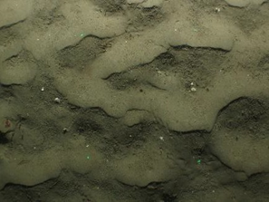
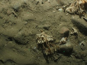
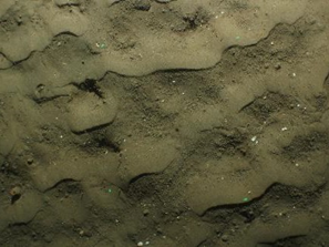
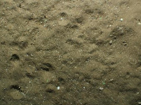
Figure 3.23: Habitat Classifications Recorded during the Environmental Survey

3.3.3.    Important Ecological Features

3.3.3. Important Ecological Features

101. In accordance with best practice guidelines developed by the Chartered Institute of Ecology and Environmental Management (CIEMM, 2022), Important Ecological Features (IEFs) have been identified for the purposes of the Array EIA Report. All potential impacts upon the IEFs due to the Array will be assessed to determine significance. According to the guidelines, importance may be determined by the quality or extent of habitats, rarity of habitats or species, and their conservation status (CIEEM, 2022). Species and habitats are considered to be IEFs if they are recognised through international or national conservation legislation or under regional or local conservation plans (e.g. Annex I and Annex II, OSPAR, National Biodiversity Plan, SBL, PMFs, etc.). The criteria used to evaluate the IEF level are presented in Table 3.20   Open ▸ .
102. The IEFs identified within the Array benthic subtidal ecology study area are presented in Table 3.21   Open ▸ , and will be taken forward for assessment within the benthic subtidal ecology EIA Chapter (volume 2, chapter 8). Within the Array EIA Report, impacts upon IEFs associated with the construction, operation and maintenance, and decommissioning of the Array will be assessed. As outlined in paragraph 96 to 100 there were several benthic subtidal habitats and species of conservation importance identified during the environmental survey of the Array benthic subtidal ecology study area. As per Table 3.19   Open ▸ , individual horse mussel were identified across the survey, however no horse mussel beds were recorded. Therefore, as only the horse mussel beds themselves are of conservation importance (PMF, SBL and OSPAR habitats), this species will not be caried forward in the IEF evaluation. Similarly, P. phosphorea (SBL) was identified in multiple sampling sites, however the closely associated sea-pen and burrowing megafauna (OSPAR) and burrowed mud (PMF) habitats were not identified. Thus, only the SBL designation for the P. phosphorea itself will be taken forward in the IEF evaluation.

Table 3.20: Criteria used to Evaluate IEFs within the Array Benthic Subtidal Ecology Study Area

Table 3.21: IEFs within the Array Benthic Subtidal Ecology Study Area